
In this section we consider a difference in two population means, \(\mu_1 - \mu_2\), under the condition that the data are not paired. The methods are similar in theory but different in the details. Just as with a single sample, we identify conditions to ensure a point estimate of the difference \(\bar
We would like to estimate the average difference in run times for men and women using the run10Samp data set, which was a simple random sample of 45 men and 55 women from all runners in the 2012 Cherry Blossom Run. Table \(\PageIndex<2>\) presents relevant summary statistics, and box plots of each sample are shown in Figure 5.6.
| men | women | |
|---|---|---|
| \(\bar \) | 87.65 | 102.13 |
| \(s\) | 12.5 | 15.2 |
| \(n\) | 45 | 55 |
The two samples are independent of one-another, so the data are not paired. Instead a point estimate of the difference in average 10 mile times for men and women, \(\mu_w - \mu_m\), can be found using the two sample means: \[\bar
Conditions for normality of \(\bar
We can quantify the variability in the point estimate, \(\bar
Distribution of a difference of sample means The sample difference of two means, \(\bar
When the data indicate that the point estimate \(\bar
Exercise \(\PageIndex<1>\) What does 95% confidence mean? Solution If we were to collected many such samples and create 95% confidence intervals for each, then about 95% of these intervals would contain the population difference, \(\mu_w - \mu_m\).
Exercise \(\PageIndex<2>\) We may be interested in a different confidence level. Construct the 99% confidence interval for the population difference in average run times based on the sample data. Solution The only thing that changes is z*: we use z* = 2:58 for a 99% confidence level. (If the selection of \(z^*\) is confusing, see Section 4.2.4 for an explanation.) The 99% confidence interval: \[14.48 \pm 2.58 \times 2.77 \rightarrow (7.33, 21.63).\] We are 99% confident that the true difference in the average run times between men and women is between 7.33 and 21.63 minutes.
A data set called baby smoke represents a random sample of 150 cases of mothers and their newborns in North Carolina over a year. Four cases from this data set are represented in Table \(\PageIndex<2>\). We are particularly interested in two variables: weight and smoke. The weight variable represents the weights of the newborns and the smoke variable describes which mothers smoked during pregnancy. We would like to know if there is convincing evidence that newborns from mothers who smoke have a different average birth weight than newborns from mothers who don't smoke? We will use the North Carolina sample to try to answer this question. The smoking group includes 50 cases and the nonsmoking group contains 100 cases, represented in Figure \(\PageIndex<2>\).
| fAge | mAge | weeks | weight | sexBaby | smoke | |
|---|---|---|---|---|---|---|
| 1 | NA | 13 | 37 | 5.00 | female | nonsmoker |
| 2 | NA | 14 | 36 | 5.88 | female | nonsmoker |
| 3 | 19 | 15 | 41 | 8.13 | male | smoker |
| \(\vdots\) | \(\vdots\) | \(\vdots\) | \(\vdots\) | \(\vdots\) | \(\vdots\) | \(\vdots\) |
| 150 | 45 | 50 | 36 | 9.25 | female | nonsmoker |
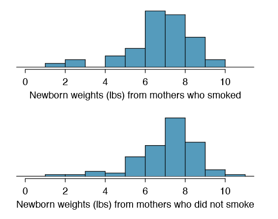
Summary statistics are shown for each sample in Table \(\PageIndex\). Because the data come from a simple random sample and consist of less than 10% of all such cases, the observations are independent. Additionally, each group's sample size is at least 30 and the skew in each sample distribution is strong (Figure \(\PageIndex\)). However, this skew is reasonable for these sample sizes of 50 and 100. Therefore, each sample mean is associated with a nearly normal distribution.
| smoker | nonsmoker | |
|---|---|---|
| mean | 6.78 | 7.18 |
| st. dev. | 1.43 | 1.60 |
| samp. size | 50 | 100 |
Solution
(a) The difference in sample means is an appropriate point estimate: \(\bar _n - \bar _s = 0.40\).
(b) Because the samples are independent and each sample mean is nearly normal, their difference is also nearly normal.
(c) The standard error of the estimate can be estimated using Equation \ref:
The standard error estimate should be sufficiently accurate since the conditions were reasonably satisfied.
If the null hypothesis from Exercise 5.8 was true, what would be the expected value of the point estimate? And the standard deviation associated with this estimate? Draw a picture to represent the p-value.
Solution
If the null hypothesis was true, then we expect to see a difference near 0. The standard error corresponds to the standard deviation of the point estimate: 0.26. To depict the p-value, we draw the distribution of the point estimate as though H0 was true and shade areas representing at least as much evidence against H0 as what was observed. Both tails are shaded because it is a two-sided test.
Compute the p-value of the hypothesis test using the figure in Example 5.9, and evaluate the hypotheses using a signi cance level of \(\alpha = 0.05.\)
Solution
Since the point estimate is nearly normal, we can nd the upper tail using the Z score and normal probability table:
\[Z = \dfrac = 1.54 \rightarrow \text = 1 - 0.938 = 0.062\]
Because this is a two-sided test and we want the area of both tails, we double this single tail to get the p-value: 0.124. This p-value is larger than the signi cance value, 0.05, so we fail to reject the null hypothesis. There is insufficient evidence to say there is a difference in average birth weight of newborns from North Carolina mothers who did smoke during pregnancy and newborns from North Carolina mothers who did not smoke during pregnancy.
Does the conclusion to Example 5.10 mean that smoking and average birth weight are unrelated?
Solution
Absolutely not. It is possible that there is some difference but we did not detect it. If this is the case, we made a Type 2 Error.
If we made a Type 2 Error and there is a difference, what could we have done differently in data collection to be more likely to detect such a difference?
Solution
We could have collected more data. If the sample sizes are larger, we tend to have a better shot at finding a difference if one exists.
When considering the difference of two means, there are two common cases: the two samples are paired or they are independent. (There are instances where the data are neither paired nor independent.) The paired case was treated in Section 5.1, where the one-sample methods were applied to the differences from the paired observations. We examined the second and more complex scenario in this section.
When applying the normal model to the point estimate \(\bar _1 - \bar _2\) (corresponding to unpaired data), it is important to verify conditions before applying the inference framework using the normal model. First, each sample mean must meet the conditions for normality; these conditions are described in Chapter 4 on page 168. Secondly, the samples must be collected independently (e.g. not paired data). When these conditions are satisfied, the general inference tools of Chapter 4 may be applied.
For example, a confidence interval may take the following form:
When we compute the confidence interval for \(\mu_1 - \mu_2\), the point estimate is the difference in sample means, the value \(z^*\) corresponds to the confidence level, and the standard error is computed from Equation \ref. While the point estimate and standard error formulas change a little, the framework for a confidence interval stays the same. This is also true in hypothesis tests for differences of means.
In a hypothesis test, we apply the standard framework and use the specific formulas for the point estimate and standard error of a difference in two means. The test statistic represented by the Z score may be computed as
When assessing the difference in two means, the point estimate takes the form \(\bar _1- \bar _2\), and the standard error again takes the form of Equation \ref. Finally, the null value is the difference in sample means under the null hypothesis. Just as in Chapter 4, the test statistic Z is used to identify the p-value.
The formula for the standard error of the difference in two means is similar to the formula for other standard errors. Recall that the standard error of a single mean, \(\bar _1\), can be approximated by
where \(s_1\) and \(n_1\) represent the sample standard deviation and sample size.
The standard error of the difference of two sample means can be constructed from the standard errors of the separate sample means:
This special relationship follows from probability theory.
Prerequisite: Section 2.4. We can rewrite Equation \ref in a different way:
Explain where this formula comes from using the ideas of probability theory. 10
This page titled 5.3: Difference of Two Means is shared under a CC BY-SA 3.0 license and was authored, remixed, and/or curated by David Diez, Christopher Barr, & Mine Çetinkaya-Rundel via source content that was edited to the style and standards of the LibreTexts platform.